mixture %>% ggplot(aes(x = normals)) +
  geom_density(aes(x = normals), color = "red") +
  geom_density(aes(x = mean_seeking_kl), color = "green") + ggtitle("The green approximation is great for IS, terrible on its own") +
  xlab("")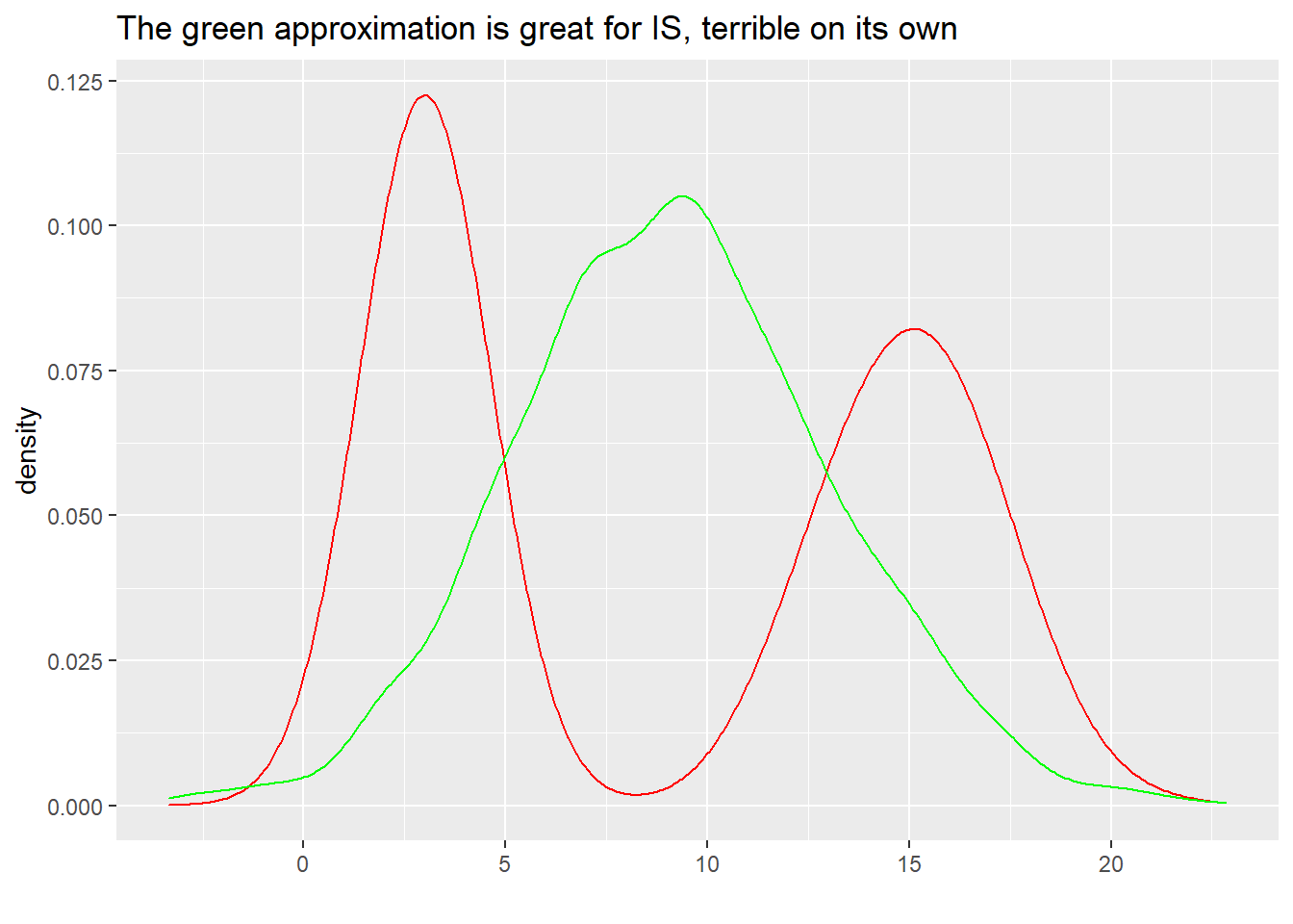
This is section 6 in my series on using Variational Inference to speed up relatively complex Bayesian models like Multilevel Regression and Poststratification without the approximation being of disastrously poor quality.
The general structure for this post and the posts around it will be to describe a problem with VI, and then describe how that problem can be fixed to some degree. Collectively, all the small improvements in these four posts will go a long way towards more robust variational inference. I’ll also have a grab bag at the end of other interesting ideas from the literature I think are cool, but maybe not as important or interesting to me as the 3 below.
In the last post we looked at normalizing flows, a way to leverage neural networks to learn significantly more expressive variational families in a way that adapt to specific problems.
In this post, we’ll explore different diagnostics for variational inference, ranging from simple statistics that are easy to calculate as we fit our approximation to solving the problem in parallel with MCMC to compare and contrast. Some recurring themes will be aiming to be precise about what constitutes failure under each diagnostic tool, and providing intuition building examples where each diagnostic will fail to do anything useful. While no single diagnostic provides strong guarantees of variational inference’s correctness on their own, taken together the tools in this post broaden our ability to know when our models fall short.
The rough plan for the series is as follows:
One logical place to start with diagnostics is to discuss what we can and can’t infer from our optimization objectives like an ELBO or CUBO.
In training a model with variational inference some common stopping rule choices are either to just run optimization for a fixed number of iterations, or to stop when relative changes in the loss have slowed, indicating convergence of the optimization to a local minimum. So we can at least look at changes in the ELBO/CUBO/other loss to know if our approximation has hit a local minimum yet.
Unfortunately, that’s about all monitoring the loss can tell us. Recall that an unknown, multiplicative constant exists in p(z,x) \propto p(z|x) that changes as reparameterize our model; thus, we can’t compare two different models on the same objective and expect their ELBO or similar loss values to be comparable. So the typical ML strategy of “which model achieves lower loss” is pretty much out here.
Also, the loss values themselves aren’t particularly meaningful: there’s no way to interpret a given ELBO as indicating a good approximation, for example. This generally stems from our bounds being bounds, not directly optimizing the quantity we want to optimize. While they’re definitely degenerate cases, there are even some fun counter examples I’ll show in a second where you can make the ELBO/CUBO arbitrarily low, while still allowing the posterior mean or standard deviation to be arbitrarily wrong!
So if we can’t just look at our loss, what can we look at? One broadly applicable diagnostic tool is \hat{k}, which we already introduced in the post on using importance sampling to improve variational inference.
As a several sentence refresher, Pareto smoothed importance sampling (PSIS) proposes to stabilize importance ratios r(\theta) used in importance sampling by modeling the tail of the distribution as a generalized Pareto distribution:
\frac{1}{\sigma} \left(1 + k\frac{r - \tau}{\sigma} \right)^{-1/k-1} where \tau is a lower bound parameter, which in our case defines how many ratios from the tail we’ll actually model. \sigma is a scale parameter, and k is a unconstrained shape parameter.
To see how this provides a natural diagnostic for importance sampling, it’s useful to know that importance sampling depends on how many moments r(\theta) has- for example, if at least two moments exist, the vanilla IS estimator has finite variance (which is obviously required, but no guarantee of performance since it might be finite but massive). The GPD has k^{-1} finite fractional moments when k > 0. Vehtari et Al. (2015) show through extensive theoretical digging and simulations that PSIS works fantastically when \hat{k} < .5. and acceptably if .5 < \hat{k} < .7. Beyond \hat{k} = .7 there the number of samples needed rapidly become impractically large.
Why should we think \hat{k} is a relevant diagnostic for variational inference? Chaterjee and Draconis (2018) showed that for a given accuracy, how big our number of samples S needs to be for importance sampling more broadly depends on how close q(x) is to p(x) in KL distance- we need to satisfy log(S) \geq \mathbb{E}_{\theta \sim q(x)}[r(\theta)log(r(\theta))] to get reasonable accuracy. So a good \hat{k} indicates importance sampling is feasible, which in turn indicates that q(x) is likely close to p(x) in KL Divergence- exactly what we’re hoping to get at!
Fleshing out the use of \hat{k} as a VI diagnostic was done by Yao et al. (2018), who generally show that high values of \hat{k} do generally map onto posterior approximations with variational inference being quite poor. This is really useful, and generally maps well on to my experience- if \hat{k} is bigger than .7, you probably need to go back to the drawing board on how you’re fitting your VI.
What I want to stress though, is that the inverse isn’t broadly true- a low \hat{k} isn’t necessarily a guarantee the VI approximation is good. Let’s look at a couple different ways this can happen.
We should keep in mind that \hat{k} is ultimately a diagnostic tool for importance sampling, and in cases where the needs of importance sampling and simple variational inference diverge, \hat{k} can give a misleading answer.
Let’s re-use an example from the importance sampling post to illustrate this. What happens if we approximate the red distribution below with the green one?
mixture %>% ggplot(aes(x = normals)) +
geom_density(aes(x = normals), color = "red") +
geom_density(aes(x = mean_seeking_kl), color = "green") + ggtitle("The green approximation is great for IS, terrible on its own") +
xlab("")
The green distribution here is a prime candidate to importance sample to approximate the red one- it coves all the needed mass, and we can massively down weight the irrelevant points in the center. On the other hand, this’d be a really, really bad variational approximation to use raw, since it has a ton of mass between the two modes which will blow up our loss. Because the needs of PSIS-based estimators and unadjusted VI diverge, \hat{k} is low, but the approximation would be pretty bad:
importance_ratios <- tibble(
q_x = rnorm(200000,9,4),
p_x = c(rnorm(100000,3,1),rnorm(100000,15,2)),
ratios = (.5*(dnorm(q_x,3,1)) + .5*(dnorm(q_x,15,2)))/dnorm(q_x,9,4))

psis_result <- psis(log(importance_ratios$ratios),
                       r_eff = NA)

psis_result$diagnostics$pareto_k
[1] -1.737515So our \hat{k} says everything is beautiful, but in reality it’s really only a happy time for PSIS, not the raw VI estimator. This ultimately isn’t the most concerning failure mode: if you do the work to calculate \hat{k}, you’re pretty much ready to use PSIS to improve your variational inference anyway. That said, this should provide intuition that \hat{k} isn’t in general super well equipped to tell you much about non-IS augmented VI.
\hat{k} inherits a common issue with most KL Divergence adjacent metrics: it’s ultimately something we evaluate locally, so if there’s a part of the posterior totally unknown to our q(x), it won’t be able to tell you what you’re missing.
We already used 1 example from the importance sampling post, so let’s keep that moving. What do you think will happen with \hat{k} with the green approximation below that misses a whole mode?
mixture %>% ggplot(aes(x = normals)) +
  geom_density(aes(x = normals), color = "red") +
  geom_density(aes(x = mode_seeking_kl), color = "green") + ggtitle("We're missing a whole mode here") +
  xlab("")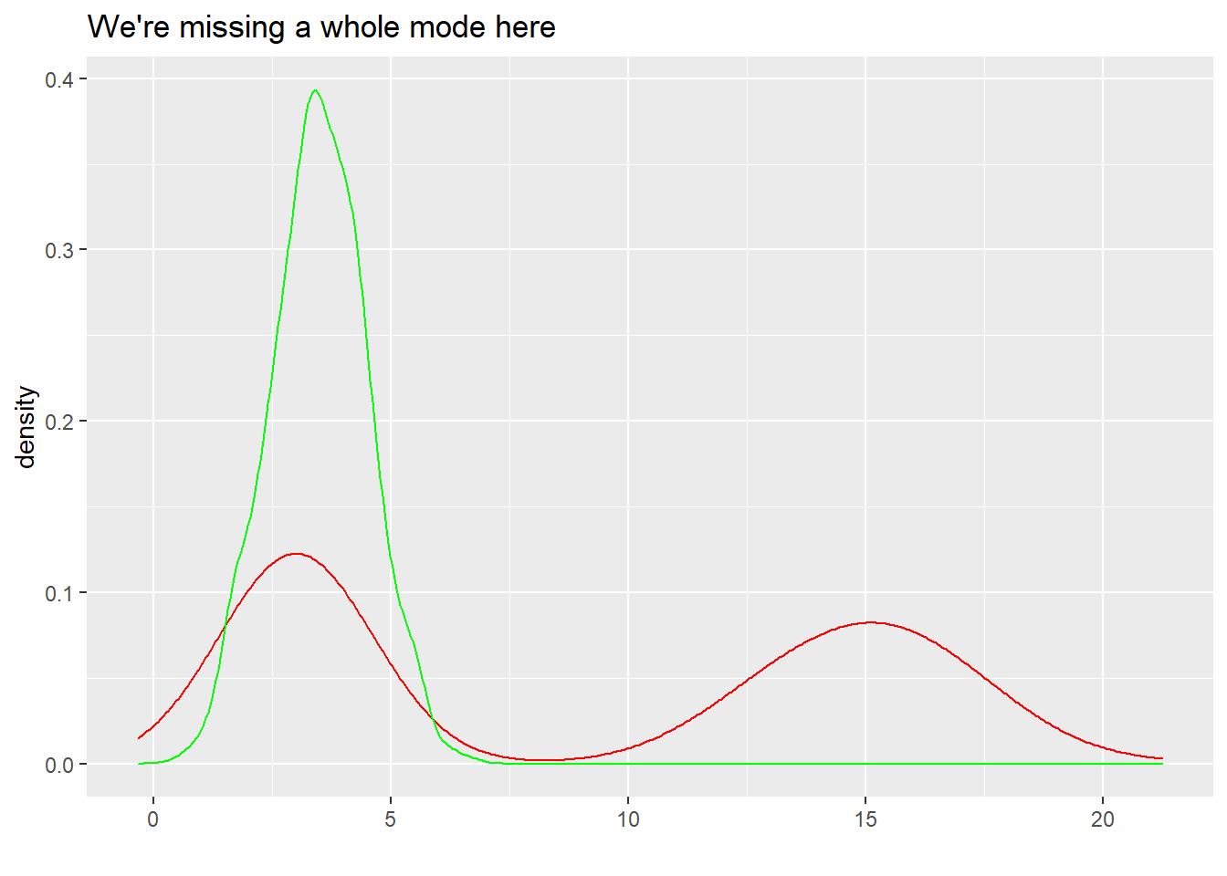
If you guessed \hat{k} will say everything is perfect when it’s not, you’re correct:
second_importance_ratios <- tibble(
q_x = rnorm(200000,3.5,1),
p_x = c(rnorm(100000,3,1),rnorm(100000,15,2)),
# Notice: these density calls are at the points defined by q(x)!
ratios = (.5*(dnorm(q_x,3,1)) + .5*(dnorm(q_x,15,2)))/dnorm(q_x,3.5,1))

psis_result_2 <- psis(log(second_importance_ratios$ratios),
                       r_eff = NA)

psis_result_2$diagnostics$pareto_k
[1] 0.07343881That’s… not great. Since we evaluate the importance ratio and thus eventually \hat{k} at the collection of values in q(x), the diagnostic has no real way to know we’re missing an entire mode, and unlike in the above case there’s no easy fix here.
Another interesting question this example raises is what happens in high dimensions, where it’s much less intuitive what “missing one or several modes” looks like. Just by increasing the sd of the normal q(x) a little in the example, we see a sudden, large increase in \hat{k};
third_importance_ratios <- tibble(
q_x = rnorm(200000,3.5,2),
p_x = c(rnorm(100000,3,1),rnorm(100000,15,2)),
ratios = (.5*(dnorm(q_x,3,1)) + .5*(dnorm(q_x,15,2)))/dnorm(q_x,3.5,2))

psis_result_3 <- psis(log(third_importance_ratios$ratios),
                       r_eff = NA)
Warning: Some Pareto k diagnostic values are too high. See help('pareto-k-diagnostic') for details.psis_result_3$diagnostics$pareto_k[1] 3.70381similar sudden shifts in \hat{k} can frequently occur as you increase the dimension of a posterior you’re approximating- intuitively, the mass you do and don’t know about becomes much harder to keep track of in high dimensions and for complex posteriors. This can lead to \hat{k} being a bit less stable than you’d like over different initializations or other slight modifications of a VI model, with this pattern being common both in my own applications and documented in several papers like Wang et al. (2023)’s testing.
A final, more conceptual problem with \hat{k} that Yao et al. (2018) point out is that it’s ultimately a diagnostic of the joint posterior, not the specific marginal or summary statistic you may ultimately care about.
Variational inference is hard: we often know that the overall posterior approximation is deeply flawed, but it may be up to the task of representing some metrics we care about correctly enough. For example, in the MRP example I introduced earlier in the series, the mean-field variational inference fit was reasonable at representing the state-level means, but garbage at pretty much anything related to uncertainty. The \hat{k} from that model was greater than 2, so we clearly know the broader posterior approximation was poor, but \hat{k} might be a false positive sign if what you really care about was just the means. For the most complicated posteriors, we should expect to spend a lot of time in this feeling of “some parts of the posterior may be good enough”, so this is a useful trap to know about.
…Let’s step back for a second. Since I introduced \hat{k} as a diagnostic with a bunch of cases where it falls short in surprising ways, I do want to emphasize it is a very useful heuristic diagnostic tool in general. Large \hat{k} tells you something is very likely wrong with your joint posterior, and that’s generally practically helpful information. Where we need to be cautious is in inferring whether the wrongness \hat{k} picks up on is something we care about, and also in remembering that low \hat{k} doesn’t provide guarantees of correctness.
So we’ve seen some limitations of using our objectives and \hat{k} as diagnostics. Let’s break out some fun propositions and examples from Huggins et al. (2020) to really drive home the need for a bound that actually makes guarantees on errors of posterior summaries we care about like means and variances.
For any t > 0, there exist (A) one dimensional, unimodal distributions q and p such that \mathrm{KL}(q \mid p) < 0.9 and \left(m_{q}-m_p\right)^2>t \sigma_p^2, and (B) one-dimensional, unimodal distributions q and p such that \mathrm{KL}(q \mid p) < 0.3 and \left(m_{q}-m_p\right)^2>t \sigma_{q}^2.
For any t \in(1, \infty], there exist one-dimensional, mean-zero, unimodal distributions q and p such that \mathrm{KL}(q \mid p)<0.12 but \sigma_p^2 \geq t \sigma_{q}^2.
So, these have some fairly scary names, huh? We can make the KL divergence pretty small, but have arbitrarily bad mean and variance approximation. How to do this? Given the examples here have to be unimodal and 1-D, they can’t be that, that weird, right?
Let Weibull (k, 1) denote the Weibull distribution with shape k>0 and scale 1. For (A), for any t>0, we can choose k=k(t), p=\operatorname{Weibull}(k, 1), and q= \operatorname{Weibull}(k / 2,1), where k(t) \searrow 0 as t \rightarrow \infty. We can just exchange the two distributions for (B).
For any t>0 we let h=h(t), p=\mathcal{T}_h (standard t distribution with h degrees of freedom), and q=\mathcal{N}(0,1) (standard Gaussian), where h(t) \searrow 2 as t \rightarrow \infty.
I won’t show it here, but the Huggins et al. paper provides a similar proposition and example for \chi^2 divergences and the CUBO bound we discussed earlier in the series, and the example has pretty much the same form.
Whenever presented with a “counterexample” to things working properly like this, it’s worth asking how broad the case’s applicability is: often counterexamples reside in the land of extremes, and we should be cautious in interpreting the result’s negative implications too broadly. There’s certainly some of that going on here, in the sense that usually a lower ELBO/CUBO will give some (if not perfect) traction in improving our posterior estimates of mean and variance. The intuitive point here though is that the bounds we optimize give no rigorous guarantees of posterior summaries we care about, even in the loosest sense.
To get some better guarantees like this, Huggins et al. (2020) propose bounds on the the mean and uncertainty estimates that arise from variational inference, which leverage the Wasserstein distance. In addition to providing actual1 bounds on quantities we care about, these bounds come at very reasonable computational cost, as they are readily computable from the bounds we already have (ELBO and CUBO) plus some additional Monte Carlo estimation and quick analytic calculation.
Let’s first discuss what the Wasserstein distance is, and then discuss the fairly involved path from our existing estimates to actually calculating the bounds.
The p-Wasserstein distance between \xi and \pi is \mathcal{W}_p(\xi, p):=\inf _{\gamma \in \Gamma(\xi, p)}\left\{\int\left\|\theta-\theta^{\prime}\right\|_2^p \gamma\left(\mathrm{d} \theta, \mathrm{d} \theta^{\prime}\right)\right\}^{1 / p} where \Gamma(\xi, p) is the set of couplings between \xi and \pi.
As a quick note on notation, I’m overloading p here a bit; given I’ve used p for our target posterior all series, I’m not going to switch that now, and calling it anything other than a p-Wasserstein distance would just be confusing to anyone who’se seen this distance before.
This looks a lot more involved than something like the KL Divergence. For example, the fact that we have an infinum over something complicated looking suggests this’ll be a real pain to calculate. As we’ll see in a second, Huggins et al. don’t actually seek to calculate it or approximate it, they seek to bound it 2.
Before we get there though, let’s seek to understand the distance and it’s properties a little better.
A good way to start unpacking this is to consider the optimal transport problem. Given some probability mass \xi(\theta) on a space X, we wish to transport it such that it is transformed into the distribution p(\theta). To provide physical intuition, this is often formulated as a problem of moving an equal amount of dirt/earth in pile \xi(\theta) to make pile \pi(\theta)- hence the name commonly used in several disciplines, the Earthmovers Distance.
Let’s say we have some non-negative cost function for moving mass from \theta to \theta^{\prime}, c(\theta,\theta^{\prime}). A single transport plan for moving from \xi(\theta) to p(\theta^{\prime}) is a function \gamma(\xi, \pi) which describes the amount of mass to move at each point. If we assume \gamma is a valid joint probability mass with marginals \xi\theta) and \pi(\theta^{\prime}) 3, then the infinitesimal mass we transport from \theta to \theta{\prime} is \gamma(\theta, \theta^{\prime}) d\theta d\theta^{\prime}, with cost
\int \int c(\theta,\theta^{\prime}) \gamma(\theta, \theta^{\prime}) d\theta d\theta^{\prime} = \int c(\theta,\theta^{\prime}) d \gamma(\theta,\theta^{\prime})
Finally getting close to something that looks like our Wasserstein distance. There are many such plans, but the one we want, the solution to the optimal transport problem, is the one with minimal cost out of all such plans.
One last point to cover to define this: what’s our cost? If the cost here is the p-distance between our \thetas, then this is the p-Wassterstein distance.
What are some properties of this distance? I already mentioned a major downside (this looks nasty to estimate in general, and indeed it is). What are the upsides of this?
Unlike the KL or \chi^2 divergences we’ve looked at before, the Wasserstein distance takes into account the metric on the underlying space! Let’s unpack that by again drawing on the optimal transport problem for intuition. The Wasserstein distance takes into account not only the differences in the values or probabilities assigned to different points in the distributions but also the actual “spatial”4 arrangement of those points.
This is a incredibly useful property because the summaries of the posterior we care about in general also rely on the underlying metric. This is basically how the arbitrarily poor mean and variance examples above work; they exploit the lack of use of an underlying metric. That allows Huggins et al. to derive one of the key results of the paper
| Theorem 3.4. If \mathcal{W}_1(q, p) \leq \varepsilon or \mathcal{W}_2(q, p) \leq \varepsilon, then \left\|m_{q}-m_p\right\|_2 \leq \varepsilon and \max _i\left|\mathrm{MAD}_{q, i}-\mathrm{MAD}_{p, i}\right| \leq 2 \varepsilon. |
| If \mathcal{W}_2(q, p) \leq \varepsilon, then for S := \sqrt{min (\left\|\Sigma_{q}\right\|_2, \left\|\Sigma_p\right\|_2)}, \max _i\left|\sigma_{q, i}-\sigma_{p, i}\right| \leq \varepsilon and \left\|\Sigma_{q}-\Sigma_p\right\|_2<2 \varepsilon(S+\varepsilon). |
A similar type of result holds for the difference between expectations of any smooth function, so this result is somewhat extensible with additional work.
This is a nice improvement over the KL or \chi^2 divergences as far as an a diagnostic, since we have some guarantees of correctness where we had literally none. I’ll return to how tight these are bounds in practice in a bit, since that’s entangled with how we can actually estimate them in the variational inference use case.
One contribution of the Huggins at al. paper is the above result, but where things get even more impressive is that they find a reasonable and practical way to bound these quantities. It’s certainly not simple, but it works.
Here’s the plan to get real bounds on our posterior summaries in full:
That’s a lot of layers of bounding, and it’s reasonable to wonder why this is needed and whether the bounds are usefully tight after such transformations. One key reason this type of bounding is so involved is that we’re using a set of scale-invariant distances to bound a scale-dependent one- we need to incorporate some notion of scale into the bounding process to make it work.
To do this, define the moment constants C_p^{\mathrm{PI}}(\xi) and C_p^{\mathrm{EI}}(\xi). For p \geq 1, \xi is p-polynomially integrable if C_p^{\mathrm{PI}}(\xi):=2 \inf _{\theta_0}\left\{\int\left\|\theta-\theta_0\right\|_2^p \xi(\mathrm{d} \theta)\right\}^{\frac{1}{p}}<\infty and that \xi is p-exponentially integrable if C_p^{\mathrm{EI}}(\xi):=2 \inf _{\theta_0, \epsilon>0}\left[\frac{1}{\epsilon}\left\{\frac{3}{2}+\log \int e^{\epsilon\left\|\theta-\theta_0\right\|_2^p} \xi(\mathrm{d} \theta)\right\}\right]^{\frac{1}{p}}<\infty
Next, with the assumption that the variational approximation q has polynomial (respectively, exponential) tails, our next result provides a bound on the p-Wasserstein distance using the \chi^2-divergence (respectively, the KL divergence).
This is saying we require at least polynomial, and ideally exponential moments for q and p, which isn’t that strenuous of a requirement. Then:
| Proposition 4.2. If p is absolutely continuous w.r.t. to q then \mathcal{W}_p(q, p) \leq C_{2 p}^{\mathrm{PI}}(q)\left[\exp \left\{\chi_2(p \mid q)\right\}-1\right]^{\frac{1}{2 p}} and \mathcal{W}_p(q, p) \leq C_p^{\mathrm{EI}}(q)\left[\mathrm{KL}(p \mid q)^{\frac{1}{p}}+\{\mathrm{KL}(p \mid q) / 2\}^{\frac{1}{2 p}}\right] |
A reasonable question here: does using the KL and \chi^2 as part of building the bounds inherit KL/\chi^2’s arbitrarily poor posterior summaries? Nope! I won’t reproduce here, but the counter examples shown above for these divergences on their own no longer work to make our estimates arbitrarily wrong.
Next step: how do we use the ELBO and CUBO to bound the KL and \chi^2 terms in the proposition above above?
We first define for any distribution \eta:
\mathrm{H}_\alpha(\xi, \eta):=\frac{\alpha}{\alpha-1}\left\{\operatorname{CUBO}_\alpha(\xi)-\operatorname{ELBO}(\eta)\right\}
Then we get:
| Lemma 4.5. For any distribution \eta such that p is absolutely continuous w.r.t. \eta- \mathrm{KL}(p \mid q) \leq \chi_\alpha(p \mid q) \leq \mathrm{H}_\alpha(q, \eta) |
By combining the lemma above and proposition from 4.2 earlier, we can bound the Wasserstein distance finally! To do this, we need all of C_p^{\mathrm{PI}}(\xi), C_p^{\mathrm{EI}}(\xi), CUBO, and ELBO. All of these are efficiently calculable much of the time (we’ll get to when it’s not soon), and largely result from things we were already calculating as promised. Great! Our combined result:
Theorem 4.6. For any p \geq 1 and any distribution \eta, if p is absolutely continuous w.r.t. q, then \mathcal{W}_p(q, p) \leq C_{2 p}^{\mathrm{PI}}(q)\left[\exp \left\{\mathrm{H}_2(q, \eta)\right\}-1\right]^{\frac{1}{2 p}} and \mathcal{W}_p(q, p) \leq C_p^{\mathrm{EI}}(q)\left[\mathrm{H}_2(q, \eta)^{\frac{1}{p}}+\left\{\mathrm{H}_2(q, \eta) / 2\right\}^{\frac{1}{2 p}}\right] .
This basically completes the process, other than some discussion of how to actually compute the quantities needed for the bounds above. The ELBO and CUBO we can compute as introduced previously in the series.
They have a good practical suggestion for a workflow given their bounds rely on CUBO, and thus on Monte Carlo estimation5. Before proceeding any further with a VI approximation, they suggest using \hat{k} < .7 as an initial diagnostic of the approximation, before calculating their bounds or leveraging importance sampling or PSIS to improve the estimate. Their point is that if \hat{k} is high, the Monte Carlo work involved in generating their bounds will be unreliable at reasonable sample sizes, and thus you won’t be able to gaurantee the bounds are useful.
A final computational point you may be wondering about is how to calculate the moment constants, C_p^{\mathrm{PI}}(\xi) and C_p^{\mathrm{EI}}(\xi). They provide a helpful example showing how to do this when q is a T distribution, and so the moments used are analytically calculable. What about when this isn’t possible? They suggest one can reasonably do this by fixing \epsilon and \theta_0 (for example, setting \theta_0 at the mean of the distribution), and sampling from q, which seems reasonable on a bit of reflection. The main reason this is worth bringing up: you don’t need a q with easy to calculate moments to make this work, which was a worry when I first saw the moment constants.
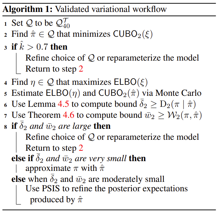
So the final, combined workflow6 they suggest is:
This was a very, very long derivation, but hopefully walking through why we would want a distance with a sense of scale and how to calculate it helped build your intuition around variational inference.
While these bounds are genuinely useful, let’s talk through some caveats and limitations of this diagnostic tool.
First, the bound really only is trustworthy when we can reliably estimate the CUBO, as I discussed above. Fortunately, as Higgins et al. note, we have an affordable way to check this in \hat{k}. Of course, we then take on the responsibility of finding a solution where we can trust \hat{k}, one which doesn’t fall into any of the blind spots the algorithm has that I discussed above. If we want to leverage the bounds, we’re also sort of forced to find a variational family that works well with the CUBO bound, even if an ELBO-based solution might work better. None of this is insurmountable, and much of the time my experience is that you probably need to change your variational family anyway if the \hat{k} for the CUBO optimized approximation is greater than .7.
The second issue here is tightness of the bounds. As you might expect, the whole “bounds via bounds of bounds” thing can result in fairly loose bounding behavior. Wang et al. (2023) show some informative examples where the bounds are anywhere from 10-1000x (!) too conservative. For example, here’s an example of theirs over Neal’s funnel:
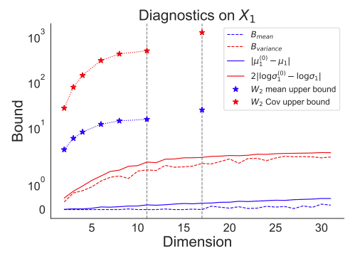
The W^2 based bounds (stars) here are 10-100x times too large compared to the true values (dashed lines). In my experience, this example and others from the paper aren’t pathological examples- the bounds are frequently this loose, especially for high dimensional and complex posteriors. Exactly what drives the achieved tightness of the bounds is fairly opaque to me; there are several stages of bounds, and it’s not really been possible to pinpoint the source of problems when the bounds are particularly loose.
However, this isn’t to say the bounds aren’t useful, far from it. In practice, especially on variance or covariance parameters, when things go off the rails, they often really go off the rails. If your variational family is nowhere near up to fitting a model, knowing you’re not within a few OOMs of reasonable values can actually be pretty helpful7. Also, these bounds provide some rigorous sense of approximation error where we previously had none, so in that sense this is a big step forward, even if they are loose.
So \hat{k} and Wasserstein bounds are both useful, but don’t tell us nearly as much as we really want to know, or do it as reliably as we’d hope. When the show isn’t going well, play the greatest hits: can we go back to using MCMC?
…Ok yeah, this feels like a bit of moving the goalposts, and in some sense it is. I motivated this whole series by saying I have models I’d like to fit where MCMC was impractically slow. But if you really want your variational approximation to look like what MCMC gives you, and do it over some summary of the posterior that isn’t a top-level mean, variance, or other simple summary, it may be the only responsible thing to do to break out your markov chains again. And things aren’t as bad as they sound here; there are a couple of ways to sanity check your VI with MCMC without committing to days of runtime.
Probably the most obvious way to use MCMC to sanity check variational inference is to not sanity check every model, just the occasional one. For example, say I was going to fit something like our MRP model to a running poll, and re-run the inferences weekly or daily. We can pretty reasonably make the leap from assuming if the variational approximation compares favorably to MCMC in the first such fit, the subsequent ones will also fit alright given the underlying data doesn’t fundamentally change in some way.
This is a pretty practical way to get the benefits of VI with the comfort MCMC gives you, as long as MCMC fits in a manageable time window. It’s just important to make sure to set up a realistic process where you spot check the occasional fit along the way, or perhaps retest with MCMC for other questions or shifts in the respondent pool that might plausibly break your model. This is the best strategy I’ve found for validating variational inference so far; even if an MCMC run can take a week or more, as long as it only has to happen once in a while that’s a totally reasonable price of admission.
…But what if you’re using variational inference because MCMC will not finish at all? This is totally possible if you have millions of data points, and/or a complex model to estimate. In this case, you may need to give MCMC a good environment to succeed in.
A simple way to do this is to subsample the full data if that’s the choking point. For example, if I have a model that I want to use variational inference to fit on millions of rows, I can reasonably infer most of the time that 100k observations will still tell me at least something useful. By fitting the subsampled data with both MCMC and variational inference, we can make sure that at least at that scale the fits align.
Another, more challenging, but perhaps more efficient way to test when MCMC is unworkably slow on the full data is through data simulation. By simulating data that contains some of the core features I’m hoping my model will understand, and only simulating a moderate amount of it, I can see if VI can capture those features the same way MCMC can. For example, if I think understanding immigration survey question responses is a complex interaction of race, education, and location, I can simulate data which has the patterns I believe exist, and see if VI does meaningfully worse than VI for that covariance structure in the model. This approach or something close to it is something mentioned by David Shor in several of his talks about Blue Rose Research’s Bayesian models which they scale to hundreds of millions of observations.
A final newer and more efficient way to gut check VI with MCMC is through Wang et al. (2023)’s TArgeted Diagnostic for Distribution Approximation Accuracy algorithm, or TADDAA8. TADDAA provides a relatively compute efficient way to bound the error of VI via MCMC. They have two main motivations for this paper: first, that many existing VI diagnostics penalize approximations that are bad in any way, not necessarily just the ways you care about most (hence, TArgeted). Realistically, for complex models, it’s not a question of if a variational approximations are worse than MCMC, it’s a question of how. Second, they note that the Wasserstein bounds we discussed earlier are often so loose as to be impractical. Again, true.
These are both sensible points, but both are really properties of MCMC, not their algorithm, so the real juice in the paper is how they bound the error efficiently. Their strategy is to fit a variational inference model, draw values, and then start many short chains of MCMC at those points. If the variational approximation to the target distribution is good, we shouldn’t expect the MCMC running for a while to change much- the points should already be in highly plausible parts of parameter space. If the approximation is less good, then if the MCMC is setup well, the chains should move towards more correct values. Even if the chains don’t reach stationarity, this can be used to provide a lower bound on the amount of approximation error a variational approximation has.
Before I discuss a few technical details, visually the idea is:
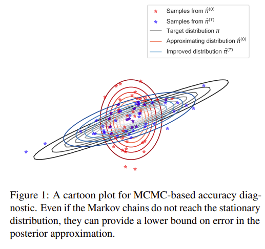
If things aren’t too poorly setup for MCMC, we can reasonably assume that the blue distribution (MCMC modified) will be between the red one (original VI posterior) and the black (true posterior). Neat!
In practice, this can work pretty well as you’d expect, and provides much tighter bounds than Wasserstein bounds given it’s a flavor of MCMC. Repeating the plot example I used earlier, notice how much closer the solid lines from the TADDAA bounds are to the dashed ones (ground truth) than the stars (denoting Wasserstein bounds):
I won’t wade too, too far into implementation details here as there a lot of them, but I do want to give enough information to discuss compute cost legibly. A first point worth raising is that “how many chains/iterations do I need” is shown by the paper to be a function of the accuracy you want on the bound- this adaptivity and ability to calculate what number of iterations you need ahead of time is convenient. Second, they’re using a lot of fairly sophisticated techniques in MCMC all together to make this efficient- strong sampling algorithms like MALA/HMC/Barker, preconditioning, and inter-chain adaptation (INCA) to adapt proposal parameters across the chains together. That’s both a great thing (this paper taught me about several new techniques around MCMC I didn’t previously know), and a bad one (to implement this for broader use there is a LOT of work to implement TADDAA efficiently9).
In their tests, all of this heavy machinery buys them some fairly impressive speed: implementing TADDAA takes from 2-18% of the gradient evaluations that the actual variational approximation takes. It’s a little opaque to me how that translates into wall time- on the one hand the many little chains are parallizeable, on the other if the number of the iterations is large that’d be the major driver of actual time this takes to run. Still, given it’s never several times VI’s compute needs like more generic MCMC would be in their tests, this seems pretty promising.
This paper is only a few months old, so I should be clear I’ve only had a bit of time to digest and play with the algorithm. If a more robust implementation became available, and the computational efficiencies they suggest are real for complex posteriors too, then this will be a fantastic new tool. They are absolutely right on the point that targeted diagnostics are valuable, and it seems like this is a way forward to getting bounds on the most relevant posterior summaries efficiently. As is, the time to set this up isn’t worth the effort versus letting simpler MCMC comparisons run for longer.
So let’s take stock of the state of variational inference diagnostics. In terms of fast to calculate solutions, there are several tools that can help us detect quite poor approximations in \hat{k} and Wasserstein bounds, but both have significant limitations. Each help detect some classes of posterior issues, but not others, and it’s a little opaque when we can strongly feel that their answers are reliable, even using both together. These feel worth running, but I’m not sure any of them are load bearing yet.
Using MCMC to validate variational approximations currently feels pretty necessary to me- the other metrics currently available can go wrong in numerous subtle and not-so-subtle ways. Of course, as this post hopefully shows, there are a lot of ways to make that validation price cheaper, from only testing one in several runs in a family of model, to using synthetic data to check results align between MCMC and VI at lower N sizes, to exploring new tools like TADDAA.
This post concludes my theoryposting streak. In the next post we’ll see if all the improvements to variational inference we’ve worked through in the past few posts buy us a better end product. We’ll finally return to trying to fit our MRP model better.
Thanks for reading. The code for this post can be found here.
Alternatively, not arbitrarily wrong.↩︎
No, we’re not winding up to define another bound like the CUBO or ELBO and optimize it like you might think. There’s an interesting little sub-literature on making calculating the Wasserstein distance (really, approximations of it) efficiently enough that we could use it for scalable Bayesian inference tasks like variational inference. I haven’t looked back at this literature in a few years, but Srivastava et al. (2018) is at least a starting point in this literature if you’re interested.↩︎
For further intuition, think about how this requirement maps onto our earth moving scenario. Integrating \gamma with respect to \theta^\prime (marginalizing) gives \xi(\theta)- physically, this means that the earth moved from point x needs to be equal to the amount starting there. The opposite marginalization gives \pi(\theta^\prime) as you’d expect. Hopefully the physical intuition of the constraints that come with this being a valid joint probability distribution make sense here; visually: ![]() {By Lambdabadger - Own work, CC BY-SA 4.0, https://commons.wikimedia.org/w/index.php?curid=64872543}↩︎
{By Lambdabadger - Own work, CC BY-SA 4.0, https://commons.wikimedia.org/w/index.php?curid=64872543}↩︎
This is imprecise, but hopefully this conveys the intuition well here: we want a distance measure that takes into account the distance between the points and how they need to be arranged to form one another, not just the values themselves.↩︎
See post 3 in the series if you want more of an introduction to this point, but the CUBO bound requires Monte Carlo (not MCMC) to calculate, which isn’t a huge computational cost when the approximation is good, but can quickly become unworkable or at least computationally tedious with bad or middling choice of variational families.↩︎
Bayesians love a good workflow.↩︎
More specifically, a common pattern is the variance estimates collapse, and collapse quite hard. Let’s say I fit a simpler model to our mrp survey example first; a lot of reasonable (even non-Bayesian) models will probably have a topline margin of errors of a couple percentage points. If the bounds on that was something like .0005% or so, that provides realistically useful news that our approximation is collapsing to weird point estimates like we saw in some poorly fit examples earlier in the series.↩︎
Fun fact: a key algorithmic detail here is any software implementation of TADDAA is that it must print “taddaa!” upon completing. Without this, users will lack a sense of magic or wonder that the algorithm otherwise instills.↩︎
They provide an implementation and replication materials here: https://github.com/TARPS-group/TADDAA. But from my early looks at this, this is more what’s needed to make the paper reproducible than a robust suite of tools for using TADDAA fully. It’s worth pointing out this is a major downside, since the other metrics I discuss all have pretty easy to use tools which implement them for general models at this point.↩︎
@online{timm2023,
  author = {Timm, Andy},
  title = {Variational {Inference} for {MRP} with {Reliable} {Posterior}
    {Distributions}},
  date = {2023-06-17},
  url = {https://andytimm.github.io/posts/Variational MRP Pt6/variational_mrp_pt6.html},
  langid = {en}
}